---
title: "Senior Freeze Proposed Policy Change"
format:
html:
toc: true
code-tools: true
code-fold: true
toc-location: left
tbl-cap-location: margin
fig-cap-location: margin
df-print: paged
---
## Summary of UIC GFRC’s Research on the Senior Freeze Exemption
The research team was asked to determine what 2025 eligibility cap for the senior freeze would be necessary to make the share of senior households eligible the same as it was when the current cap was put in place in 2017.
The Senior Freeze is a property tax relief program that locks in assessed values for eligible seniors to prevent them from being priced out of their homes. The income cap of \$65,000 has not been raised since 2017 and is not pegged to inflation. Thus, many seniors have been “bumped off the rolls” due to inflation.
The research team found that raising the eligibility cap to \$85,000 approximates the 2017 eligibility threshold accounting for inflation. Moreover, explicitly linking the eligibility cap to inflation will prevent seniors from falling off the rolls in the future.
The research team also found that raising the income cap to \$85,000 would have a negligible effect on taxing districts’ revenue-neutral tax rate. Composite tax rates would rise 0.05 percentage points at most, even in the South suburbs with the largest property tax rates.
## Supporting Code and Background Info
"Low-income Senior Citizens Assessment Freeze Homestead Exemption (SCAFHE) A person qualifies for this exemption if the person
- is at least 65 years old;\
- has a total household income of \$65,000 or less; and\
- meets certain other qualifications.
This exemption "freezes" the senior citizen's property's equalized assessed value the year that the senior citizen qualifies for the exemption. The property's equalized assessed value does not increase as long as qualification for the exemption continues. The tax bill may still increase if any tax rates are increased or if improvements are added that increase the value of the property.
This exemption allows senior citizens who meet the qualifications to elect to maintain the equalized assessed value (EAV) of their homes at the base year EAV and prevent any increase in that value due to inflation. The amount of the exemption benefit is determined each year based on (1) the property's current EAV minus the frozen base year value (the property's prior year's EAV for which the applicant first qualifies for the exemption), and (2) the applicant's total household maximum income limitation.
Each year applicants must file a Form PTAX-340, Low-income Senior Citizens Assessment Freeze Homestead Exemption Application and Affidavit, with the Chief County Assessment Office.
[(35 ILCS 200/15-170)](http://www.ilga.gov/legislation/ilcs/fulltext.asp?DocName=003502000K15-170) Additional Info - [Illinois.gov](https://tax.illinois.gov/localgovernments/property/taxrelief.html#:~:text=This%20program%20allows%20persons%2065%247%2C500)
### Using PUMA Data
```{r warning=FALSE, message=FALSE, results='hide'}
library(tidyverse)
library(ipumsr)
library(tigris)
library(srvyr)
library(naniar)
library(survey)
knitr::opts_chunk$set(message = FALSE, warning = FALSE)
# PUMA shapefiles
pumasIL2020 <- pumas("IL", cb=T, year=2020)
pumasIL2020 <- pumasIL2020 |>
mutate(County = ifelse(
str_sub(GEOID20, 1, 5) == "17031", "Cook", NA),
YEAR="2023") |>
select(-c(ALAND20, AWATER20, STATEFP20, AFFGEOID20, LSAD20, STUSPS20, ST_NAME20)) |>
rename(GEOID=GEOID20,
puma = PUMACE20,
puma_area = NAMELSAD20)
pumasIL2018 <- pumas("IL", cb=T, year=2018)
pumasIL2018 <- pumasIL2018 |>
mutate(County = ifelse(
(str_sub(GEOID10, 1, 5) == "17034" |
str_sub(GEOID10, 1, 5) == "17035") == TRUE, "Cook", NA) ,
YEAR="2018") |>
select(-c(ALAND10, AWATER10, STATEFP10, AFFGEOID10, LSAD10 ) ) |>
rename(GEOID = GEOID10,
puma = PUMACE10,
puma_area = NAME10
)
pumas <- rbind(pumasIL2018, pumasIL2020) |>
mutate(uniqueid = paste0(puma, "_", YEAR),
puma_area = str_remove_all(puma_area, " PUMA")) |>
filter(County == "Cook")
ddi <- read_ipums_ddi("../inputs/usa_00026.xml")
data2018 <- read_ipums_micro(ddi) |>
mutate(PUMA = str_pad(PUMA, 5,side = "left", pad="0"),
YEAR = as.character(YEAR)
) |>
select(YEAR, PUMA, PERWT, HHWT, AGE, SEX, PERNUM, HHINCOME, INCEARN, VALUEH, OWNERSHP, STRATA,
CLUSTER, HHTYPE, SERIAL, SAMPLE) |>
left_join(pumasIL2018, by = c("PUMA" = "puma", "YEAR"))
ddi <- read_ipums_ddi("../inputs/usa_00025.xml")
data2023 <- read_ipums_micro(ddi) |>
select(YEAR, PUMA, PERWT, HHWT, AGE, SEX, PERNUM, HHINCOME, INCEARN, VALUEH, OWNERSHP, STRATA,
CLUSTER, HHTYPE, SERIAL, SAMPLE) |>
mutate(PUMA = str_pad(PUMA, 5, side = "left", pad="0"),
YEAR = as.character(YEAR)) |>
left_join(pumasIL2020, by = c("PUMA" = "puma", "YEAR"))
data <- rbind(data2018, data2023)
data <- data |>
mutate(
VALUEH = ifelse(VALUEH == 9999999, NA, VALUEH),
HHINCOME = ifelse(HHINCOME == 9999999 | HHINCOME == 9999998, NA, HHINCOME)
)
data <- data |>
mutate(age_cat =
case_when(AGE < 24 ~ "16to24",
AGE > 24 & AGE < 35 ~ "25to34",
AGE > 34 & AGE < 45 ~ "35to44",
AGE > 44 & AGE < 55 ~ "45to54",
AGE > 54 & AGE < 65 ~ "55to64",
AGE > 64 ~ "65+"),
sex_cat = case_when(SEX == 1 ~ "Male",
SEX == 2 ~ "Female"))
# #check coding make sure it is the same for both censuses
# data <- data |> mutate(white = if_else(RACE ==1, 1, 0),
# black = if_else(RACE ==2, 1, 0),
# asian = if_else(RACE %in% c(4,5,6), 1, 0),
# otherrace = if_else(RACE %in% c(3,7,8,9),1,0))
```
```{r}
#| include: false
head(data$HHTYPE)
summarytools::freq(data$HHTYPE)
head(data$OWNERSHP)
```
```{r include=FALSE}
data |>
filter(YEAR == "2023") |>
group_by(SERIAL) |> ## Household ID number
summarize(multi_peep = n(),
HHWT = mean(HHWT),
owned = max(OWNERSHP),
hhinc = max(HHINCOME),
house_value = max(VALUEH),
oldest = max(AGE),
youngest = min(AGE)) |>
# filter(multi_peep > 1) |>
arrange(desc(multi_peep) )
data |>
filter(YEAR == "2023") |>
#group_by(SERIAL) |> ## Household ID number
summarize(obs = n(),
HHWT = sum(HHWT),
PERWT = sum(PERWT))
```
38,112 obs in data for Cook County downloaded from IPUMS. summed HHWT representing 5,029,986 households and 5,086,576 individuals.
10,461 unweighted household observations with more than 1 person in them. 17,119 unweighted household observations in IPUMs data for Cook County.
```{r}
#| include: false
obs_perPUMA <- data |>
group_by(YEAR, PUMA, age_cat) |>
dplyr::summarize(weightedcount=sum(HHWT), #weighted
unweightedcount = n()) |>
arrange(PUMA)
obs_perPUMA
obs_perPUMA |>
select(-unweightedcount) |>
pivot_wider(names_from = "age_cat", values_from = "weightedcount")
# 1 = OWNED, 2 = RENTED, 3 = N/A
obs_perPUMA<- data |>
filter(PERNUM == 1) |> # only use one person from each household, the "householder"?
group_by(PUMA, age_cat, OWNERSHP ) |>
dplyr::summarize(
hhs_wghted = sum(HHWT),
unweightedcount = n()) |>
arrange(PUMA)
obs_perPUMA
```
```{r}
#| layout-ncol: 2
# INCEARN
# AGE
# VETSTAT
# HHINCOME
data |> filter(YEAR == 2018) |>
ggplot() + geom_histogram(aes(x=HHINCOME, weight = HHWT))
data |> filter(YEAR == 2023) |>
ggplot() + geom_histogram(aes(x=HHINCOME, weight = HHWT))
data |> filter(YEAR == 2018) |>
ggplot() + geom_histogram(aes(x=INCEARN, weight = PERWT))
data |> filter(YEAR == 2023) |>
ggplot() + geom_histogram(aes(x=INCEARN, weight = PERWT))
```
```{r}
# inc_quantiles <- survey::svyquantile(~HHINCOME, design=HHdesign,
# quantiles = c(0, 0.1, 0.2, 0.3, 0.4, 0.5, 0.6, 0.7, 0.8, 0.9, 1) ,
# na.rm=TRUE, ci = FALSE )
# inc_quantiles
#
# 0 0.1 0.2 0.3 0.4 0.5 0.6 0.7 0.8 0.9 1
# [1,] -7900 21600 40000 58700 77000 97000 120000 148400 185000 261000 1744000
#
## numbers used for income breaks are calculated in Income Deciles section.
# created now so that the variable exists in the joined dataset before creating the survey design object
data <- data |>
mutate(
## current senior freeze threshold!
below_freeze = ifelse(HHINCOME >= 65000, "Not Eligible", "Eligible"),
new_freeze = ifelse(HHINCOME >= 85000, "Not Eligible", "Eligible"),
)
# filter to household head only so households are counted
# multiple times for each person in the household
HHdesign <- survey::svydesign(id = ~SERIAL, nest=TRUE, strata = ~STRATA, weights = ~HHWT, data = data|> filter(PERNUM==1))
```
### Comparisons
```{r}
#| label: fig-current-income-threshold-during2018
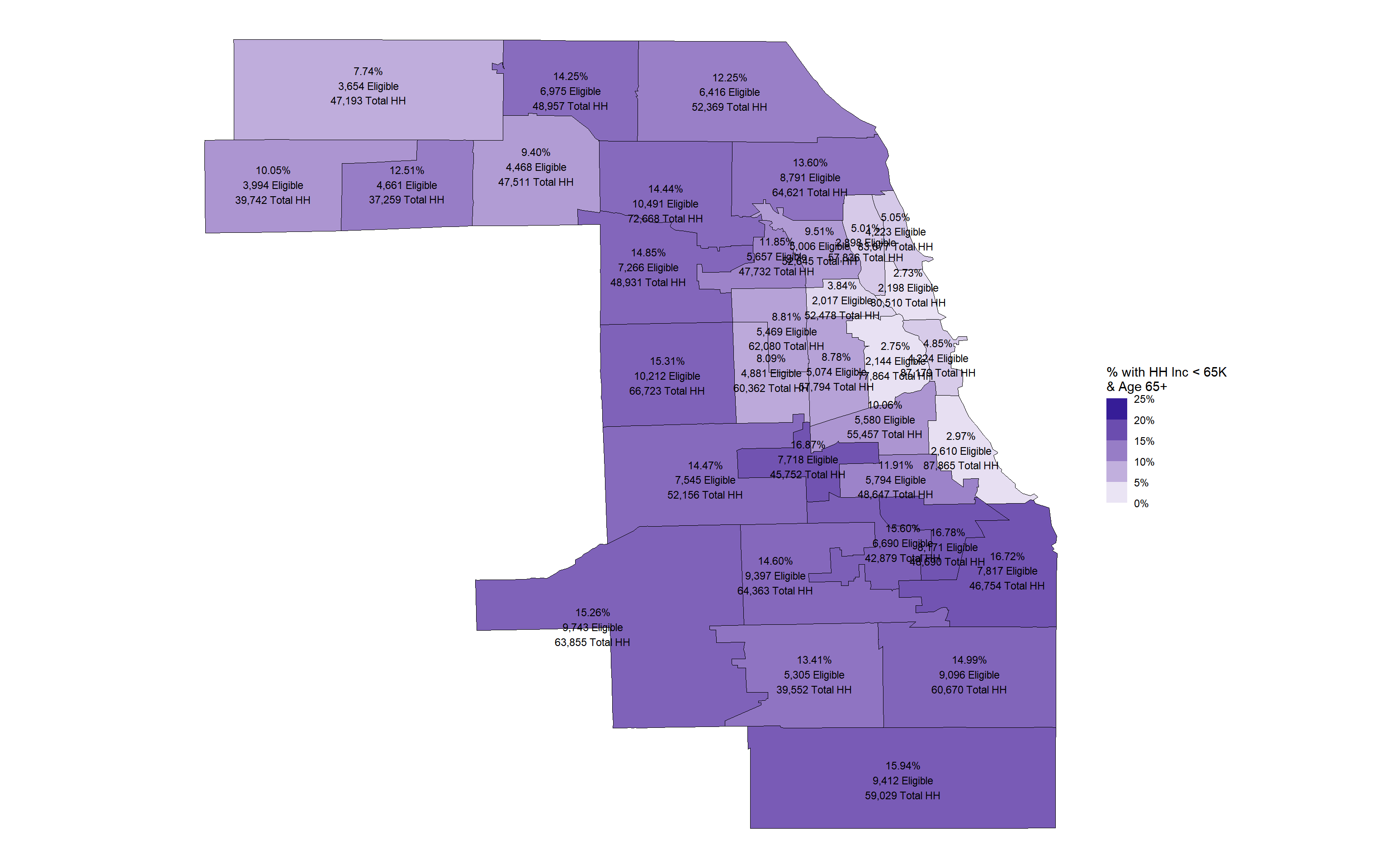
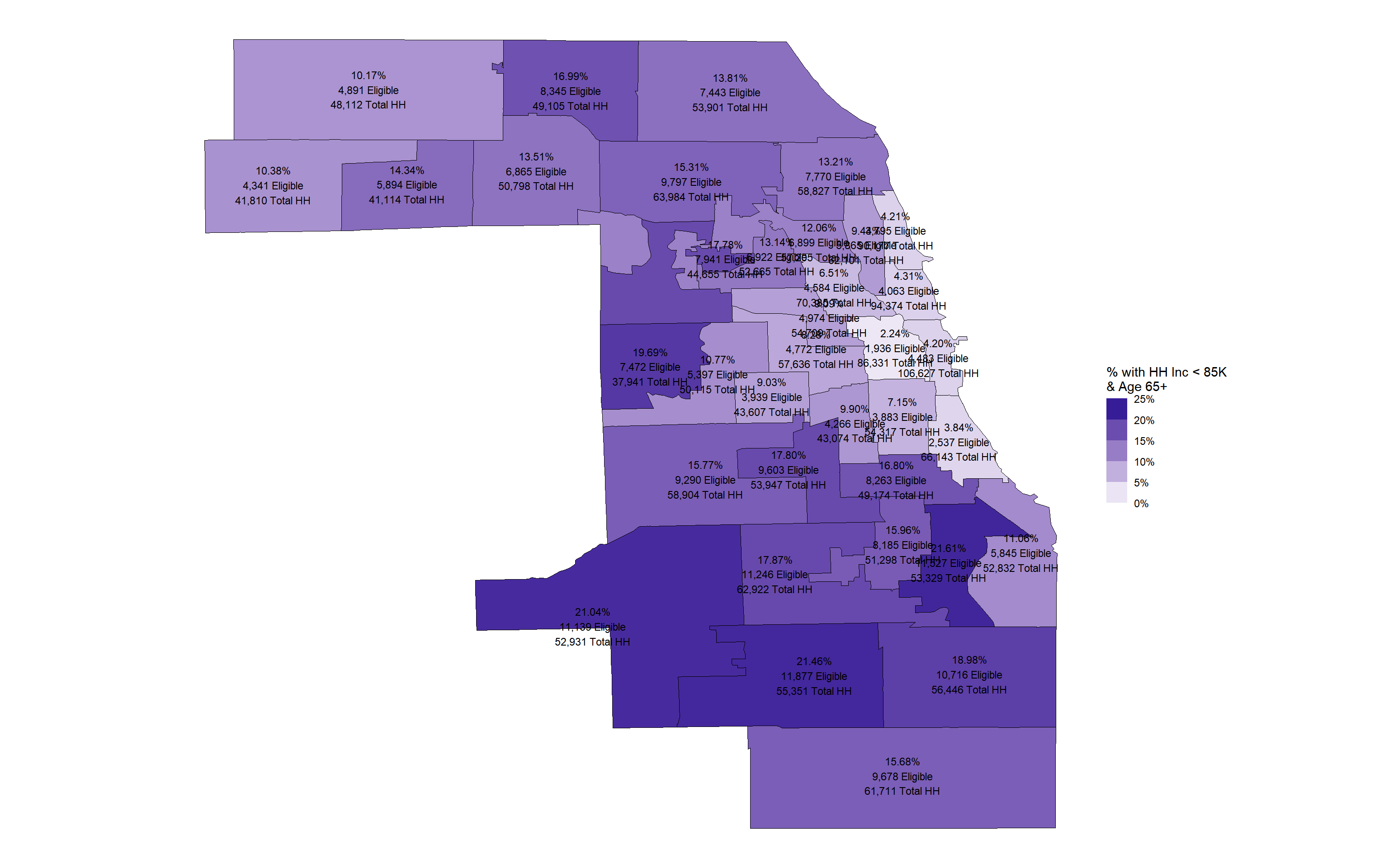
#| fig-cap: "Share of all Own. Occ. Households 65+ w/ HH incomes < $65K in 2018 compared to all Owner Occupied Households 65+ with household incomes less than 85K in 2023. Shows number of households eligible for the Low-Income Senior Freeze Exemption in 2018, when the income threshold was last updated and the percent that would be eligible if the income threshold were increased to $85,000 based on 2023 data."
#| fig-height: 10
#| fig-width: 16
#| column: screen-inset
#| layout-ncol: 2
incometable <- svytable(~ YEAR + PUMA + OWNERSHP + age_cat + below_freeze, design = HHdesign)
mapPUMAboth <- incometable |>
as_tibble() |>
mutate(PUMA = str_pad(PUMA, 5, side= "left", pad = "0"),
) |>
group_by(YEAR, PUMA) |>
mutate(
Prop = n/sum(n),
Total = sum(n)
)
mapPUMAboth <- mapPUMAboth |>
filter(below_freeze == "Eligible" & age_cat == "65+" & OWNERSHP == 1 &
YEAR == 2018) |>
inner_join(pumas, by = c("PUMA" = "puma", "YEAR"))
current_policy_in2018<- ggplot(mapPUMAboth,
aes(fill = Prop,
geometry = geometry,
label = paste0(
scales::percent(Prop, accuracy = 0.01), "\n",
scales::comma(n), " Eligible", "\n",
scales::comma(Total), " Total HH")
#" ", "frac(", n, ",", Total, ")"
)) +
geom_sf(color = "black")+
geom_sf_text(size = 3) +
theme_void() +
theme(axis.ticks = element_blank(), axis.text = element_blank())+
scale_fill_binned(
high = "darkblue", low = "white",
limits = c(0, 0.25),
breaks = c(0, 0.05, 0.10, 0.15, 0.20, 0.25),
# show.limits=TRUE,
#nice.breaks=FALSE,
labels=scales::percent,
name = "% with HH Inc < 65K\n& Age 65+")
current_policy_in2018
incometable <- svytable(~ YEAR + PUMA + OWNERSHP + age_cat + new_freeze, design = HHdesign)
mapPUMAboth <- incometable |>
as_tibble() |>
mutate(PUMA = str_pad(PUMA, 5, side= "left", pad = "0"),
) |>
group_by(YEAR, PUMA) |>
mutate(
Prop = n/sum(n),
Total = sum(n)) |>
filter(new_freeze == "Eligible" & age_cat == "65+" & OWNERSHP == 1
& YEAR == 2023) |>
inner_join(pumas, by = c("PUMA" = "puma", "YEAR"))
new_policy_in2023 <- ggplot(mapPUMAboth,
aes(fill = Prop,
geometry = geometry,
label = paste0(
scales::percent(Prop, accuracy = 0.01), "\n",
scales::comma(n), " Eligible", "\n",
scales::comma(Total), " Total HH")
)) +
geom_sf(aes(geometry = geometry), color = "black")+
geom_sf_text(size = 3) +
# labs(title = "Share of all Own. Occ. Households 65+ w/ HH incomes < $85K",
# subtitle = "Eligible for the Senior Freeze Exemption if Household Income increased to $85K") +
theme_void() +
theme(axis.ticks = element_blank(), axis.text = element_blank())+
scale_fill_binned(high = "darkblue", low = "white",
limits = c(0,0.25),
breaks = c(0, 0.05, 0.10, 0.15, 0.20, 0.25),
#show.limits=TRUE,
#nice.breaks=FALSE,
labels=scales::percent,
name = "% with HH Inc < 85K\n& Age 65+")
new_policy_in2023
```
### Current Policy - \$65K
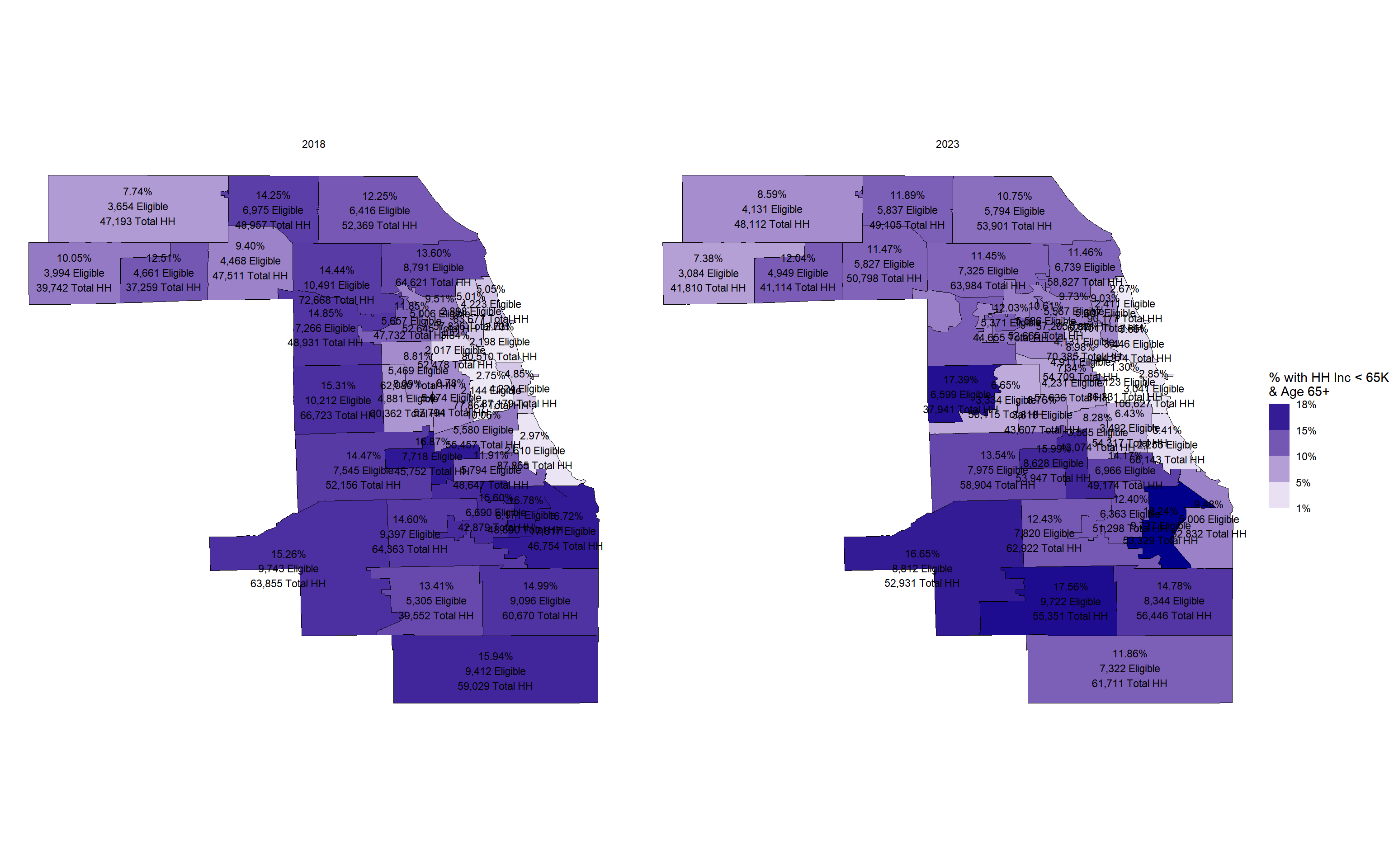
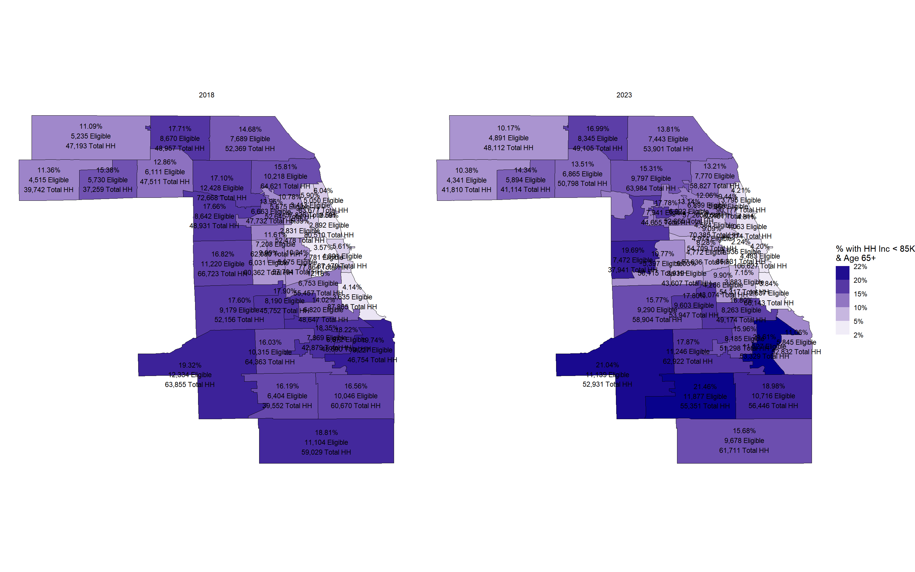
Bloom and Rich Townships had 542 more senior households but 2000+ fewer households eligible for senior freeze. Adjusting the senior freeze income threshold to \$85K would make the share of senior, owner-occupied households comparable to 2018 when the policy was adjusted last (\~ 16% owner occupied, 65+ households in these two townships were eligible in 2018). Worth and Calumet Townships gained 1300 senior, owner occupied households from 2018 to 2023 but had 1400+ fewer eligible households. Share of owner occupied senior households eligible went from 14.6% in 2018 to 12.4% in 2023.
Wheeling Township had 479 fewer senior households in 2023 than in 2018, but 1138 fewer households eligible for the senior freeze. Northfield and New Trier Townships had 679 fewer senior households and 622 fewer households eligible for senior freeze exemption.
All numbers are based off of ACS 5-year estimates downloaded from the IPUMS USA database.
```{r}
#| label: tbl-changeinseniorhouseholds
#| tbl-caption: "Change in Owner occupied senior households"
incometable <- svytable(~ YEAR + PUMA + OWNERSHP + age_cat, design = HHdesign)
mapPUMAboth <- incometable |>
as_tibble() |>
mutate(PUMA = str_pad(PUMA, 5, side= "left", pad = "0"),
) |>
group_by(YEAR, PUMA) |>
mutate(
Prop = n/sum(n),
Total = sum(n)
)
mapPUMAboth <- mapPUMAboth |>
filter(age_cat == "65+" & OWNERSHP == 1) |>
inner_join(pumas, by = c("PUMA" = "puma", "YEAR"))
mapPUMAboth |>
ungroup() |>
group_by(puma_area) |>
pivot_wider( id_cols = c(puma_area), names_from = "YEAR", values_from = "n") |>
mutate(change = `2018`-`2023`) |>
select(change, puma_area# Prop, puma_area
) |>
arrange(desc(change)) |>
DT::datatable(rownames = FALSE)
```
```{r}
#| label: tbl-currenteligible-change
#| fig-caption: "Change in number of people eligible from 2018 to 2023, based on the $65,000 household income threshold for the senior freeze."
incometable <- svytable(~ YEAR + PUMA + OWNERSHP + age_cat + below_freeze, design = HHdesign)
mapPUMAboth <- incometable |>
as_tibble() |>
mutate(PUMA = str_pad(PUMA, 5, side= "left", pad = "0"),
) |>
group_by(YEAR, PUMA) |>
mutate(
Prop = n/sum(n),
Total = sum(n)
)
mapPUMAboth <- mapPUMAboth |>
filter(below_freeze == "Eligible" & age_cat == "65+" & OWNERSHP == 1) |>
inner_join(pumas, by = c("PUMA" = "puma", "YEAR"))
mapPUMAboth |>
ungroup() |>
group_by(puma_area) |>
pivot_wider( id_cols = c(puma_area), names_from = "YEAR", values_from = "n") |>
mutate(change = `2018`-`2023`) |>
select(change, puma_area# Prop, puma_area
) |>
arrange(desc(change)) |>
DT::datatable(rownames = FALSE)
```
```{r}
#| label: fig-current-income-threshold
#| fig-cap: "Share of all Own. Occ. Households 65+ w/ HH incomes < $65K. Shows number of households eligible for the Low-Income Senior Freeze Exemption in 2018, when the income threshold was last updated, and the number of households that are eligible in tax year 2023."
#| fig-height: 10
#| fig-width: 16
#| column: screen-inset
current_policy <- ggplot(mapPUMAboth,
aes(fill = Prop,
geometry = geometry,
label = paste0(
scales::percent(Prop, accuracy = 0.01), "\n",
scales::comma(n), " Eligible", "\n",
scales::comma(Total), " Total HH")
#" ", "frac(", n, ",", Total, ")"
)) +
geom_sf(color = "black")+
geom_sf_text(size = 3) +
#labs(title = "Share of all Own. Occ. Households 65+ w/ HH incomes < $65K",
# subtitle = "Currently Eligible for Senior Freeze"#,
# caption = "n represents the number of households eligible") +
theme_void() +
theme(axis.ticks = element_blank(), axis.text = element_blank())+
# theme(legend.position = "bottom")+
scale_fill_binned(high = "darkblue", low = "white",
guide = guide_coloursteps(show.limits = TRUE),
labels=scales::percent,
name = "% with HH Inc < 65K\n& Age 65+") +
facet_wrap(~YEAR)
current_policy
```
### New Policy - \$85K
```{r}
HHdesign <- survey::svydesign(id = ~SERIAL, nest=TRUE, strata = ~STRATA, weights = ~HHWT, data = data |> filter(PERNUM==1))
```
```{r byage, include=FALSE}
agetable <- svytable(~YEAR + PUMA + age_cat, design = HHdesign)
mapPUMAboth <- agetable |>
as_tibble() |>
mutate(PUMA = str_pad(PUMA, 5, side= "left", pad = "0")) |>
group_by(YEAR, PUMA) |>
mutate(
Prop = n/sum(n)) |>
filter(age_cat =="65+") |>
ungroup() |>
left_join(pumas, by = c("PUMA" = "puma", "YEAR" = "YEAR"))
#mapPUMAboth |> select(YEAR, countyFIP, PUMA, Prop, n, NAME10)
figure <- ggplot(mapPUMAboth, aes(fill = Prop)) +
geom_sf(aes(geometry = geometry), color = "black")+
labs(title = "Senior Households are up to 30% of all households in some areas",
subtitle = "Percent of PUMA Households in 2023 that are 65+") +
theme_void() +
theme(axis.ticks = element_blank(), axis.text = element_blank())+
scale_fill_binned(
high = "darkblue", low = "white",
guide = guide_coloursteps(show.limits = TRUE),
labels=scales::percent,
name = "% HH 65+") +
facet_wrap(~YEAR)
figure
```
```{r below85K, include = FALSE}
incometable <- svytable(~ YEAR + PUMA + new_freeze, design = HHdesign)
mapPUMAboth <- incometable |>
as_tibble() |>
mutate(PUMA = str_pad(PUMA, 5, side= "left", pad = "0")) |>
group_by(YEAR, PUMA) |>
mutate(
Prop = n/sum(n)) |>
filter(new_freeze == "Eligible")|>
left_join(pumas, by = c("PUMA" = "puma", "YEAR" = "YEAR"))
#mapPUMAboth |> select(YEAR, countyFIP, PUMA, Prop, n, NAME10)
figure5c <- ggplot(mapPUMAboth, aes(fill = Prop)) +
geom_sf(aes(geometry = geometry), color = "black")+
labs(title = "Share of ALL households below 85K") +
theme_void() +
theme(axis.ticks = element_blank(), axis.text = element_blank())+
scale_fill_binned(high = "darkblue", low = "white",
guide = guide_coloursteps(show.limits = TRUE),
labels=scales::percent,
name = "% with HH Inc < 85K ") +
facet_wrap(~YEAR)
figure5c
```
```{r over65andunder85K, include=FALSE, eval=FALSE}
incometable <- svytable(~ YEAR + PUMA + age_cat + new_freeze, design = HHdesign)
mapPUMAboth <- incometable |>
as_tibble() |>
mutate(PUMA = str_pad(PUMA, 5, side= "left", pad = "0"),
# new_freeze = ifelse(hhincdecile_w >= 5, "Not Eligible", "Eligible")
) |>
group_by(YEAR, PUMA) |>
mutate(
Prop = n/sum(n)) |>
filter(new_freeze == "Eligible" & age_cat == "65+") |>
inner_join(pumas, by = c("PUMA" = "puma", "YEAR"))
#mapPUMAboth |> select(YEAR, PUMA, Prop, n, age_cat)
figure5c <- ggplot(mapPUMAboth, aes(fill = Prop)) +
geom_sf(aes(geometry = geometry), color = "black")+
labs(title = "Share of all households 65+ w/ HH incomes < $85K") +
theme_void() +
theme(axis.ticks = element_blank(), axis.text = element_blank())+
scale_fill_binned(high = "darkblue", low = "white",
guide = guide_coloursteps(show.limits = TRUE),
labels=scales::percent,
name = "% with HH Inc < 85K ") + facet_wrap(~YEAR)
figure5c
```
```{r}
#| label: fig-proposed-income-threshold
#| fig-cap: "Share of all Own. Occ. Households 65+ w/ HH incomes < $85K."
#| fig-height: 10
#| fig-width: 16
#| column: screen-inset
incometable <- svytable(~ YEAR + PUMA + OWNERSHP + age_cat + new_freeze, design = HHdesign)
mapPUMAboth <- incometable |>
as_tibble() |>
mutate(PUMA = str_pad(PUMA, 5, side= "left", pad = "0"),
) |>
group_by(YEAR, PUMA) |>
mutate(
Prop = n/sum(n),
Total = sum(n)) |>
filter(new_freeze == "Eligible" & age_cat == "65+" & OWNERSHP == 1) |>
inner_join(pumas, by = c("PUMA" = "puma", "YEAR"))
new_policy <- ggplot(mapPUMAboth,
aes(fill = Prop,
geometry = geometry,
label = paste0(
scales::percent(Prop, accuracy = 0.01), "\n",
scales::comma(n), " Eligible", "\n",
scales::comma(Total), " Total HH")
)) +
geom_sf(aes(geometry = geometry), color = "black")+
geom_sf_text(size = 3) +
# labs(title = "Share of all Own. Occ. Households 65+ w/ HH incomes < $85K",
# subtitle = "Eligible for the Senior Freeze Exemption if Household Income increased to $85K") +
theme_void() +
theme(axis.ticks = element_blank(), axis.text = element_blank())+
scale_fill_binned(high = "darkblue", low = "white",
guide = guide_coloursteps(show.limits = TRUE),
labels=scales::percent,
name = "% with HH Inc < 85K\n& Age 65+") +
facet_wrap(~YEAR)
new_policy
```
### PTAXSIM Part
> REMEMBER: **senior freeze exemption is called `exe_freeze`** in ptaxsim. The senior exemption is called `exe_senior`
```{r make-sf-pins}
#| eval: false
ptaxsim_db_conn <- DBI::dbConnect(RSQLite::SQLite(),
"./ptaxsim.db/ptaxsim-2023.0.0.db")
pins <- DBI::dbGetQuery(
ptaxsim_db_conn,
"SELECT *
FROM pin
WHERE exe_freeze > 0
"
)
sf_pins <- pins |> distinct(pin) |> select(pin)
# pulls all data for all years for PINs that had a freeze exemption at least one year
pins <- DBI::dbGetQuery(
ptaxsim_db_conn,
glue_sql(
"SELECT *
FROM pin
WHERE pin IN ({sf_pins$pin*})"
,
.con = ptaxsim_db_conn
))
pins <- pins |>
group_by(pin) |>
arrange(pin, year) |>
mutate(years_with_sfexe = sum(exe_freeze > 0),
gain_lose = case_when(
years_with_sfexe == 18 ~ "Always had SF Exe",
exe_freeze > 0 & lag(exe_freeze) == 0 ~ "Gained SF Exe",
exe_freeze == 0 & lag(exe_freeze) > 0 ~ "Lost SF Exe",
TRUE~"No Change"
))
write_rds(pins, "inputs/senior_freeze_pins.RDS")
```
```{r}
#| label: tbl-read-in-seniorfreezepins
#| tbl-cap: "Counts of those that gained or lost senior freeze exemptions per year
#| "
pins <- read_rds("../inputs/senior_freeze_pins.RDS")
# n_distinct(pins$year)
table(pins$year, pins$gain_lose)
```
10 million+ observations for pin-years for senior exemption.\
5,879,046 pin-year combos for **senior freeze exemption**.
583,163 distinct pins had senior exemption at least 1 year.\
328,836 had the senior freeze exemption at least 1 year.
50,241 properties had the senior exemption every year from 2006 to 2023. 7,075 PINs had the senior freeze exemption every year from 2006 to 2023.
```{r}
#| label: tbl-sfpins-in2023
#| tbl-cap: "Counts of those that gained or lost senior freeze exemptions in 2023 compared to 2022"
pins |> filter(year == 2023) |> group_by(gain_lose) |> summarize(n = n())
```
```{r}
pins |>
group_by(year) |>
summarize(had_SF_exe = sum(exe_freeze>0)) |>
ggplot() +
geom_line(aes(x=year, y = had_SF_exe)) +
geom_vline(aes(xintercept=2017), color= "red", lwd=1) +
labs(y= "# PINs", x="", title = "PIN Count: Senior Freeze Exemption", caption = "Tax Year 2017 was the first year for senior freeze exemption increase")+
theme_bw()
```
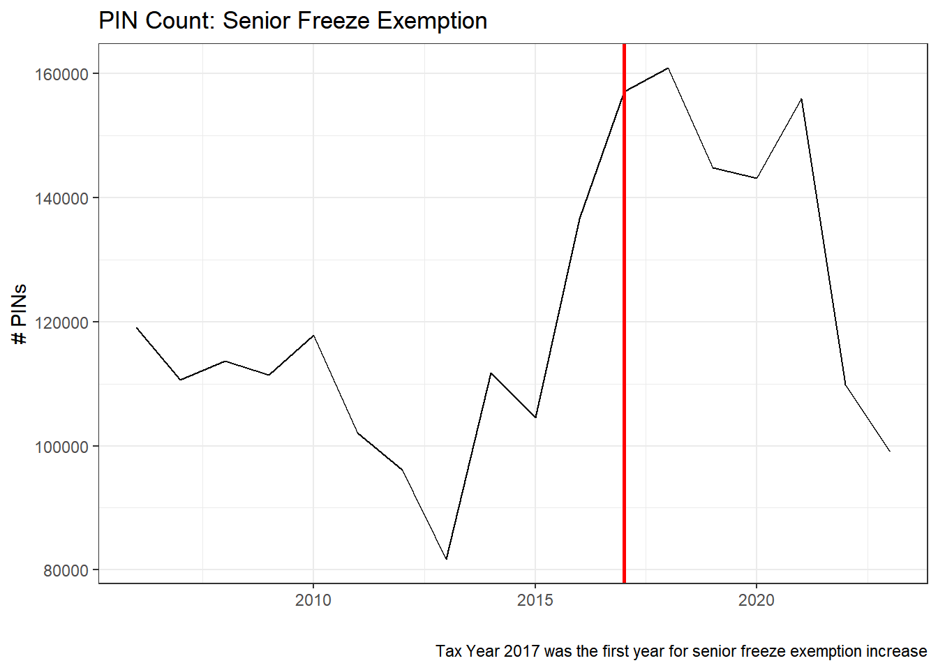
Senior freeze exemption was last increased and reflected in Tax Year 2017. [Civic Federation](https://www.civicfed.org/iifs/blog/new-state-law-increases-cook-county-property-tax-homestead-exemptions)
```{r pinsthatdidnthave_exeforallyears}
pins2 <- pins |> ungroup() |> filter(years_with_sfexe != 18)
table(pins2$years_with_sfexe[pins2$year==2023])
```
```{r }
#| label: tbl-lost-SF
#| tbl-cap: "PINs that lost SF exemption and hadit for more than 5 years"
#|
pins2 |> ungroup() |> filter(gain_lose=="Lost SF Exe" & years_with_sfexe > 5) |> arrange(pin)
```
```{r }
#| label: tbl-billchange
#| tbl-cap: "Average tax bill across the years of when a PIN had the SF exemption compared to when it did not have the SF exemption. PINs had exemption for different number of years so it is not a perfect comparison for average taxbills."
pins2 |>
group_by(pin)|>
summarize(bill_wo_exemp = mean(tax_bill_total[gain_lose== "Lost SF Exe"]),
bill_w_exemp = mean(tax_bill_total[gain_lose == "Gained SF Exe"])) |>
mutate(avg_diff = bill_wo_exemp - bill_w_exemp)
```
#### **Looking at taxbills over time for a couple random pins:**
For PIN 01011000430000, their bill went up \$2500 from 2010 to 2011 and increased \$1400 from 2013 to 2014.
```{r}
#| code-fold: false
pins |> filter(pin == "01011000430000") # lost exemption in 2011 and 2014
pins |> filter(pin == "01011240370000") # lost exemption in 2019 and 2023
# bill went up $1400 in 2023
pins |> filter(pin == "02112010020000")
```
```{r}
#| label: tbl-pins-gained-sf
#| tbl-cap: "PINs that gained a SF exemption."
pins2 |> ungroup() |> filter(gain_lose=="Gained SF Exe") |> arrange(pin)
```